
Why SELECT Is Not Executed First in SQL (Beginner Guide)
Learn the real SQL execution order step by step. Understand why SELECT runs last, avoid common mistakes, and ace SQL interviews with clarity.
If you have ever written a SQL query, you know the drill. You start by typing SELECT, list out the columns you want, and then proceed to figure out where the data is coming from using FROM. It is the most natural way to express what you want. After all, when you go to a restaurant, you order your food (the SELECT part) before the chef goes to the kitchen to gather the ingredients (the FROM part). You do not start by telling the waiter to go to the fridge, look for tomatoes, bring them to the counter, and then ask for a salad.
But what if I told you that the database engine works in the exact opposite way?
One of the most common stumbling blocks for developers—both junior and mid-level—is the disconnect between how a SQL query is written (the lexical order) and how it is actually executed by the database engine (the logical processing order). This fundamental misunderstanding leads to hours of frustrating debugging, confusing error messages about missing column aliases, and inefficient queries that bring applications to a crawl. You might find yourself staring at an error message complaining that a column you literally just typed in the SELECT clause does not exist in the GROUP BY clause.
In this comprehensive guide, we are going to tear down a SQL query and rebuild it from the perspective of the database engine. We will explore the true logical execution order of SQL, step by step. By the end of this article, you will not only write better, more performant queries, but you will also understand exactly why the database behaves the way it does. You will never look at a SELECT statement the same way again.
Declarative vs. Imperative Programming: The Heart of the Matter
To understand why SQL execution order is inverted from its written order, we first need to understand the nature of the SQL language itself and the philosophy behind its design.
Most general-purpose programming languages you use on a daily basis—like C#, Java, Python, or JavaScript—are imperative languages. In imperative programming, you provide the computer with a step-by-step list of instructions to execute in order to achieve a goal. You manage the state, the loops, the exact flow of control, and you manually direct the computer on how to allocate memory. You are micromanaging the machine. If you want to find all employees making over $100,000, you write a loop, check each object, and push it to a new array.
SQL (Structured Query Language), on the other hand, is a declarative language. When you write SQL, you are describing the desired result, not the steps required to achieve it. You declare what you want the final dataset to look like, what conditions the data must meet, and how it should be grouped. You leave the heavy lifting of figuring out how to get that data to the database's internal system known as the Query Optimizer.
The Query Optimizer is a highly sophisticated piece of software that analyzes your declarative SQL statement, evaluates various execution strategies (using statistics, indexes, and heuristics), and generates a Physical Execution Plan. It decides whether to use a hash join, a nested loop join, an index seek, or a full table scan.
However, before the optimizer can do its magic, the database engine must interpret your query according to a strict standard known as the Logical Processing Order. This conceptual framework dictates how the intermediate result sets—often called virtual tables—are built, filtered, and passed from one step to the next. The logical processing order is the contract that ensures your query returns the correct results, regardless of the physical execution plan chosen by the optimizer.
The Complete Logical Processing Order
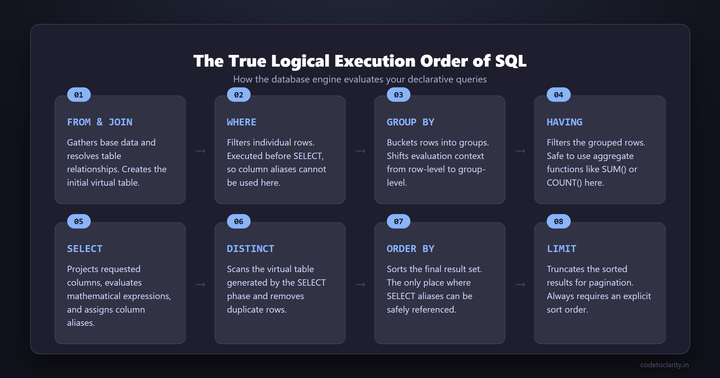
While you write a query starting with SELECT, the logical evaluation of a standard SQL query actually begins with the FROM clause. Here is the standard logical processing order for a SQL SELECT statement:
FROMONJOINWHEREGROUP BYWITH CUBEorWITH ROLLUP(if applicable)HAVINGSELECTDISTINCTORDER BYOFFSET/FETCH/TOP/LIMIT
Let’s break down each of these steps in detail to understand exactly what happens to your data as it flows through the SQL engine. We will look at the virtual tables created at each stage and understand how data transforms from raw disk blocks into the pristine result set on your screen.
Phase 1: Gathering the Data (FROM, ON, JOIN)
Before you can filter, group, or select any data, you must first define where the data is coming from. The database needs a foundation to work with. This is why the logical execution begins here.
Step 1: FROM
The FROM clause is the starting point of any query. The database engine looks at the tables specified here. If multiple tables are specified without explicit join logic (e.g., FROM TableA, TableB), the engine performs a Cartesian product (Cross Join). This means every single row in TableA is matched with every single row in TableB. If TableA has 1,000 rows and TableB has 1,000 rows, the resulting virtual table (let's call it VT1) will have 1,000,000 rows!
This is why proper schema design is the foundation of all database performance. If you want to ensure your tables are designed optimally before even writing queries, you must start with a solid schema. A poorly designed schema will cause massive virtual tables and kill performance right at step one. You can read more about this in our guide on Why Your Database Is Slow (And It’s Not the Query).
Step 2: ON
Next, the database applies the join condition specified in the ON clause to the virtual table generated by the FROM phase. Only the rows for which the ON condition evaluates to TRUE are inserted into a new virtual table (VT2). This step filters out non-matching rows early in the join process.
For example, ON TableA.Id = TableB.TableAId ensures that we only keep rows where the foreign key matches the primary key. If a row evaluates to FALSE or UNKNOWN (because of a NULL value), it is discarded from VT2. The ON clause is your first line of defense against data explosion.
Step 3: JOIN (Outer Joins)
If you specified an Outer Join (such as a LEFT JOIN or RIGHT JOIN), the rows from the preserved table that were filtered out during the ON phase are now added back into the virtual table (creating VT3). For these restored rows, the columns originating from the non-preserved table are filled with NULL values.
At the end of this phase, the database has gathered all the raw data necessary for your query. The joins have been resolved, and we have a massive virtual table containing every column from every joined table.
Phase 2: Row-Level Filtering (WHERE)
Once the base dataset is assembled, the database engine moves to the WHERE clause. This is the first place where we begin discarding data we do not care about based on business rules.
Step 4: WHERE
The WHERE clause applies a search condition to each individual row of the virtual table generated by the previous phase. Only rows that evaluate to TRUE are allowed to pass through to the next virtual table (VT4).
Here is a crucial limitation that confuses many beginners: You cannot use column aliases created in the SELECT clause inside the WHERE clause.
Take a look at this commonly written, but entirely invalid, query:
SELECT
    EmployeeId,
    BaseSalary + Bonus AS TotalCompensation
FROM
    Employees
WHERE
    TotalCompensation > 100000; -- THIS WILL FAIL!
Why does this fail? Look at the execution order. The WHERE clause (Step 4) is evaluated long before the SELECT clause (Step 8). When the database engine processes the WHERE clause, the TotalCompensation alias literally does not exist yet in its memory. To fix this, you must repeat the expression:
SELECT
    EmployeeId,
    BaseSalary + Bonus AS TotalCompensation
FROM
    Employees
WHERE
    (BaseSalary + Bonus) > 100000; -- THIS WORKS!
Additionally, you cannot use aggregate functions like COUNT() or SUM() in the WHERE clause because grouping has not occurred yet. The database is still thinking in terms of individual rows, not grouped buckets.
Pro Tip on Sargability: When writing WHERE clauses, you must ensure your conditions are "SARGable" (Search Argument ABLE). This means writing conditions that allow the database to use indexes. If you wrap a column in a function (e.g., WHERE YEAR(HireDate) = 2026), the database cannot use an index on HireDate because the function fundamentally alters the data before comparison, forcing a full table scan. Instead, you should write WHERE HireDate >= '2026-01-01' AND HireDate < '2027-01-01'.
Phase 3: Aggregation (GROUP BY and HAVING)
Now that we have filtered our individual rows, the database can start summarizing the data. This is where we shift from thinking about rows to thinking about groups.
Step 5: GROUP BY
The GROUP BY clause takes the rows from the previous virtual table and groups them based on the unique values in the specified columns. It creates a new virtual table (VT5) where each group is represented by a single row.
This is a massive paradigm shift in the query's execution. Before the GROUP BY clause, the database was operating on a row-by-row basis. After this step, the database is operating on a group-by-group basis. Because of this, any subsequent clauses (like HAVING or SELECT) can only reference columns that are part of the GROUP BY clause or columns wrapped in aggregate functions. If you try to select a column that is not grouped and not aggregated, the database throws an error because it doesn't know which row's value to display for the group.
Step 6: Rollups and Cubes
If you are using advanced analytical grouping features like WITH CUBE or WITH ROLLUP, the database engine generates super-aggregate rows (like subtotals and grand totals) and appends them to the virtual table here. This is incredibly useful for generating multi-dimensional reports directly in the database without needing complex application-side logic.
Step 7: HAVING
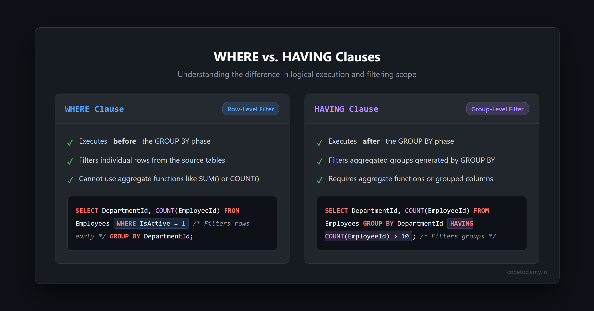
This brings us to one of the most common SQL interview questions of all time: "What is the difference between WHERE and HAVING?"
The HAVING clause is essentially the WHERE clause for groups. It applies a filter condition to the grouped rows generated by the GROUP BY clause. Only groups that evaluate to TRUE are passed along to the next step.
Because HAVING is executed after GROUP BY, it is perfectly valid to use aggregate functions here.
SELECT
    DepartmentId,
    COUNT(EmployeeId) AS EmployeeCount,
    SUM(BaseSalary) AS TotalPayroll
FROM
    Employees
WHERE
    IsActive = 1                -- Filters individual rows BEFORE grouping
GROUP BY
    DepartmentId                -- Creates the groups
HAVING
    COUNT(EmployeeId) > 10;     -- Filters the groups AFTER grouping
If you find yourself struggling with query performance due to massive aggregations, consider reading our guide on SQL Query Optimization: Tips to Speed Up Your Database to learn how indexes can dramatically speed up grouping and filtering operations.
Phase 4: Projecting the Results (SELECT)
We have finally reached the clause that we typed first! We have a virtual table of groups (or rows, if no grouping was applied), and we are ready to pick the columns we want to see.
Step 8: SELECT
The SELECT clause defines the final structure of the result set. Up until this point, the database has been passing around virtual tables containing all the columns from the underlying base tables. Now, it projects only the columns, expressions, and aggregates that you explicitly requested.
During this phase, several important things happen:
- Mathematical expressions are evaluated across the rows or groups.
- String concatenations are performed.
- Column aliases (using the
ASkeyword) are finally assigned and become available for subsequent steps. - Window functions (like
ROW_NUMBER(),RANK(), orLEAD()) are calculated.
Because window functions are calculated during the SELECT phase, you cannot use them in a WHERE clause to filter rows. If you need to filter based on a window function (for example, finding the top 3 highest paid employees per department), you must use a Common Table Expression (CTE) or a derived table to force the database to execute the SELECT clause first, and then apply a WHERE clause to the result.
This is also a great moment to address why SELECT * is considered a cardinal sin in production environments. Even if the database has narrowed down the rows via WHERE and JOIN conditions, SELECT * forces the database engine to serialize and transmit every single column across the network to your application. This bloats memory usage, increases network latency, and prevents the optimizer from using highly efficient "covering indexes". Always explicitly name the columns you need.
To understand the official specifications of how the SELECT statement operates and all its intricacies, you can review the authoritative documentation on the Logical Processing Order of the SELECT statement by Microsoft.
Phase 5: Refinement (DISTINCT and ORDER BY)
With our columns chosen and aliases assigned, we now polish the final output to make it exactly what the client requested.
Step 9: DISTINCT
If the DISTINCT keyword is present, the database scans the virtual table generated by the SELECT phase and removes duplicate rows. Because DISTINCT requires sorting or hashing the entire result set, it can be an extremely expensive operation.
As a general best practice, never use DISTINCT as a band-aid for poor joins that are multiplying your data unexpectedly. If you have duplicates, find the root cause in your JOIN conditions rather than slapping DISTINCT on the SELECT clause. It covers up bad data logic and destroys performance.
Step 10: ORDER BY
The ORDER BY clause takes the unique, filtered, grouped, and projected rows and sorts them according to your specifications.
Because ORDER BY executes after the SELECT clause, this is the first and only place in a standard SQL query where you can reference the column aliases you created in the SELECT list.
SELECT
    FirstName + ' ' + LastName AS FullName,
    HireDate
FROM
    Employees
ORDER BY
    FullName ASC; -- This works perfectly!
Sorting is another heavily resource-intensive task. If the data is not naturally sorted by an index, the database engine must perform an explicit sort operation. If you are ordering millions of rows, the database may not have enough RAM to hold the dataset and will have to spill the operation to disk (like TempDB in SQL Server), slowing down your query significantly. Always try to sort only when absolutely necessary for the presentation layer, or ensure you have appropriate indexes covering your sort columns.
Phase 6: Pagination (LIMIT / OFFSET / TOP)
The final step in the logical execution order is restricting the number of rows returned to the client application.
Step 11: OFFSET / FETCH / TOP / LIMIT
Depending on your specific relational database management system (RDBMS), you will use clauses like TOP (SQL Server), LIMIT (PostgreSQL, MySQL), or standard OFFSET / FETCH to truncate the result set.
This phase takes the fully sorted data from the ORDER BY step and returns only the specified subset of rows. It is critical to note that if you are using pagination features, you should always include an ORDER BY clause. Without an explicit sort order, relational databases do not guarantee the order of returned rows. This means your paginated results will be unpredictable and inconsistent, potentially showing the same row on page 1 and page 2 simply because the database decided to read pages from disk in a different sequence.
Why Understanding This Makes You a Better Developer
You might be thinking, "This is great theory, but does it actually matter in my day-to-day coding? Do I really need to memorize this list?" The answer is a resounding yes.
When you internalize the true order of SQL execution, several fundamental things change about how you write code:
- Debugging Becomes Logical: When a query fails with an "Invalid column name" error on an alias, you immediately know it is because you tried to reference it in a clause (like
GROUP BYorWHERE) that executes before the alias is created. You stop guessing and start fixing. - Performance Improves: You start filtering data as early as possible. You realize that a restrictive
WHEREclause reduces the number of rows that must be processed by expensiveGROUP BYandORDER BYoperations. You write leaner, meaner queries. - Advanced SQL Unlocks: You begin to understand why Common Table Expressions (CTEs) and subqueries are necessary. They force the database to complete the logical execution of one query block so that you can filter on its computed aliases or window functions in an outer query.
Furthermore, understanding query execution helps you design more resilient systems. When you are modifying data concurrently, understanding the exact moment data is read versus written is crucial. To dive deeper into ensuring data integrity across complex operations, read our complete guide on SQL Transactions Explained: Master the ACID Properties. By mastering how the engine processes reads, you are better equipped to handle writes.
The Physical Reality vs. Logical Theory
Before we conclude, it is important to add a quick disclaimer about the real world. The sequence we just covered is the logical processing order. It is the conceptual model that guarantees the correctness of your query's output. It is how you must think when you write the query.
However, under the hood, the database's Query Optimizer is incredibly smart. It generates a physical execution plan that may completely reorder these steps if it determines that a different approach will produce the exact same result much faster.
For example, if you have a highly selective WHERE clause on a massive table, and an index exists on that column, the optimizer might jump straight to the index to fetch the matching rows before it even looks at the rest of the FROM or JOIN conditions. Alternatively, the optimizer might push GROUP BY operations down below a JOIN if it reduces the data volume early in the pipeline.
The beauty of SQL is that you do not need to worry about the physical execution plan for basic querying. As long as you write your SQL assuming the logical processing order is strictly followed, the database guarantees that your results will be accurate, no matter what shortcuts the optimizer takes behind the scenes.
Final Thoughts
The mismatch between how we write SQL and how it executes is one of the language's most enduring quirks. We write SELECT first because, to a human, the shape of the desired output is the most important part of the question. We think, "I need the total sales by region" (SELECT Region, SUM(Sales)), and then we specify the source (FROM Orders).
But to a computer, you cannot shape data until you have found it, filtered it, and grouped it. It is a completely logical, mechanical process.
The next time you sit down to write a complex SQL query, do not just type it out from top to bottom. Trace it through logically. Start in your mind at the FROM clause, apply your JOINs, filter with WHERE, bucket your data with GROUP BY, filter the buckets with HAVING, project your columns with SELECT, and finally sort it with ORDER BY.
When you align your mental model with the database engine's logical processing order, the mysteries of SQL disappear, and you transform from someone who just writes queries into someone who truly engineers data. Your queries will be faster, your code cleaner, and your bugs significantly fewer.

Kishan Kumar
Software Engineer / Tech Blogger
A passionate software engineer with experience in building scalable web applications and sharing knowledge through technical writing. Dedicated to continuous learning and community contribution.